Feb 08, 2021
by Christopher Anderson
A new set of cloud computing resources and geospatial analytics systems have dramatically simplified how we work with large ecological datasets. These tools support rapid, on-the-fly spatial analyses and can be used to generate rich, interactive visualizations that make working with spatial data easier and more fun.
It wasn’t always this way. In our experience as spatial ecologists, and for many others, managing spatial data was burdensome and frustrating. The files are big, it’s easy to lose track of datasets & it’s hard to share and collaborate on projects. And handling projections is always a nightmare.
There are good and complicated technical reasons for why working with spatial data has been so hard for so long. But also: we’re trying to explore the forest. This should be cool and fun! And the tools we use to do so should be as well.
So we designed each component of the Forest Observatory around public-facing cloud computing resources and open geospatial standards to make it easy to access, analyze & visualize our data. This post describes some of the standards we’ve adopted as well as some examples for how to index and analyze our data on other platforms.
We’ll review:
We’ll also review how to use the CFO python library to work with these resources. I’ve included a set of code snippets below, which are from this example jupyter notebook.
Some notes on the CFO API
You can now install the cfo package via pip install cfo instead of getting it directly from GitHub. Hooray!
You’ll still need to sign up for an account on forestobservatory.com to use the API, which is free for non-commercial use. Forest Observatory data can still be used commercially—just get in touch.
And if you’ve signed up for an account, please make sure you’ve read the terms of use. As hip-hop fans know, you’ve gotta read the label.
Cloud-optimized geotiffs
For most users, COG files are no different from regular geotiffs. They’re still tifs, and can be read by neary all the same software systems. But they have a couple of neat advantages.
First is that they can be quickly read and analyzed from cloud storage platforms. That means you don’t have to download a whole file to your local machine when you only need a subset of data. This is technically suppored for regular geotiffs too, but it’s typically much slower: you often have to read a lot of extra data to get the subset you need. Regular geotiffs aren’t often optimized to handle arbitrary subsets.
The second advantage is that COGs reduce server-side costs for the organizations that host free spatial data (like us!). We’re responsible for network and data egress costs, and serving data in COG format means we’re minimizing the number of https requests as well as the amount of data read from cloud storage.
The jupyter notebook demo works through some examples of how to query individual pixel values and clip/download data using vector files. Here are a few lines of code using gdal to retrieve the tree height value from a single pixel from cloud asset:
import cfo
from osgeo import gdal

# initialize the cfo api
forest = cfo.api()

# search for the 2020 high res canopy height asset ID
ch_ids = forest.search(
    geography="California",
    metric="CanopyHeight",
    year=2020,
    resolution=3,
)

# this returns a 1-element list, but we need a string
ch_id = ch_ids.pop()

# get the virtual file path
ch_path = forest.fetch(ch_id, gdal=True)

# set the lat/lon coordinates of the tree (from google maps)
pine_coords = [-122.46776, 37.7673]

# since these are in lat/lon, convert to pixel locations
x, y = pixel_project(ch_path, pine_coords, epsg=4326)

# then read the value at that location
ch_ref = gdal.Open(ch_path, gdal.GA_ReadOnly)
height = ch_ref.ReadAsArray(x, y, 1, 1)
In running the notebook, you should find that the height of the tree at that coordinate (a Monterey Pine at the entrance of the San Francisco Botanic Garden) is 28 meters tall.
I left out a few things to simplify this post (like defining the pixel_project function)—follow along in the notebook for the full code.
Google Earth Engine
Earth Engine is a tremendously cool and useful platform for analyzing huge amounts of geospatial data. It’s pretty popular now thanks to an active user community and development team, and it has been cited in over 2,500 scientific articles. We use it all the time.
We also use Google Cloud Platform as our cloud service provider, which has several points of integration with Earth Engine. We host Forest Observatory data in a publicly-accessible cloud storage bucket and, now that Earth Engine supports reading COGs from several cloud storage locations, we can read our data directly in Earth Engine.
The jupyter notebook contains examples using the Earth Engine Python API and the CFO API to read datasets, display maps, and query pixel values. Here’s a sample for loading our high resolution Canopy Cover maps and very simply computing change over time:
# get the canopy cover asset IDs
cc_ids = forest.search(
    geography="California",
    metric="CanopyCover",
    resolution=3,
)
cc_ids.sort()

# get the bucket paths for where each file is stored
cc_bucket_paths = [forest.fetch(cc_id, bucket=True) for cc_id in cc_ids]

# read them as earth engine images
cc_2016 = ee.Image.loadGeoTIFF(cc_bucket_paths[0])
cc_2020 = ee.Image.loadGeoTIFF(cc_bucket_paths[1])

# compute the difference between years
change = cc_2020.subtract(cc_2016)

# mask changes below a change detection threshold.
thresh = 15
mask = change.gt(thresh).Or(change.lt(-thresh))
change = change.mask(mask)
Then, with more code than I care to paste here, we create a map using folium to display these canopy cover and change datasets inline. Here’s a screenshot from the notebook:
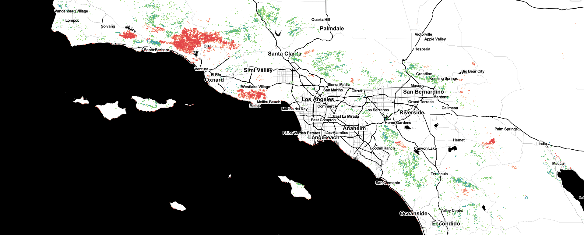
This map shows patterns of Canopy Cover change from 2016 to 2020, mapped at the scale of the individual tree, with canopy loss in warm colors and canopy growth in cool ones. Showing changes in the mountains around southern California, distinct footprints of recent wildfires and woody encroachment express how wildfire hazards, species habitat & regeneration patterns dynamically shift over time.
You can generate your own interactive map to zoom in and explore the patterns using the jupyter notebook we provided. It’s pretty neat, I swear.
SpatioTemporal Asset Catalogs
Until recently, ecology was a fairly data-scarce discipline. Field plots and species occurrence records were sparsely and opportunistically collected, and access was fragmented among research groups. But several advances in the past decade—the deployment of hundreds of earth observing sensors, the consolidation and standardization of open ecological data, and increased access to open software and computing resources—have significantly reduced the ecological data gap. What should we make of all this new information? And how should we organize it?
We founded Salo to address the former question: our mission is to use global ecological data to identify conservation opportunities, monitor ecosystem health & predict environmental change. But I digress.
STAC was developed to address the latter question. It is, in short, a metadata tagging system designed to index spatially and temporally explicit datasets. STAC supports querying data catalogs by time and location, is built around web/https-friendly json formats, supports consistent tagging processes (e.g. specifying spatial resolution), and generally makes it easy to find and understand cloud-based spatial data. It can be used to catalogue data locally, too.
For people familiar with Google Earth Engine’s ImageCollection paradigm, STAC catalogs and collections are organized in a very similar fashion, and can queried in similar ways.
This is particularly useful for working with satellite data, which generates tons of spatially-explicit image data over time. It is likewise useful for the California Forest Observatory, which uses these regularly-collected data for monitoring ecosystem health over time.
So we adopted the STAC framework, and Forest Observatory data is now accessible via the following STAC catalog:
https://storage.googleapis.com/cfo-public/catalog.json
You can query this catalog using pystac, which is demonstrated in the notebook. Here’s a quick subset:
# set and read the catalog
catalog_url = "https://storage.googleapis.com/cfo-public/catalog.json"
catalog = pystac.Catalog.from_file(catalog_url)

# what's in it?
print(catalog.description)

# iteratively retrieve the catalog items
print("Catalog contents:")
print(catalog.describe())
This returns:
The California Forest Observatory is a data-driven forest monitoring system that maps the drivers of wildfire behavior across the state-including vegetation fuels, weather, topography & infrastructure-from space.

Catalog contents:
* <Catalog id=forest-observatory>
    * <Collection id=vegetation>
      * <Item id=California-Vegetation-CanopyBaseHeight-2016-Summer-00010m>
      * <Item id=California-Vegetation-CanopyBaseHeight-2017-Summer-00010m>
      * <Item id=California-Vegetation-CanopyBaseHeight-2018-Summer-00010m>
...
You can query the catalog for all the available CFO datasets. We’ll be sure to keep this updated as we publish more and more data.
Check the jupyter notebook for more detail and more examples, or just load the collection in the STAC software of your choice. The easiest way I’ve found to browse catalogs via the web is through stacindex.org. I found pystac is pretty easy to learn, too (check their introductory demo notebook).
Closing
We designed the Forest Observatory to support the next generation of geospatial software tools to make it easy to understand and analyze environmental change using high resolution data.
California’s ecosystems are changing rapidly, and we’re trying to do everything we can to keep pace. This includes providing insights into how and why these systems are changing.
We hope you find the tools and data we’ve created to be useful in your pursuit of the same goals.
Bonus content
At the header of this post is a picture I took of Half Dome from the sky. I like this photo because it captures the sweeping beauty, complexity & range of California’s mountain forests.
And although this is a much flatter depiction, here’s a map of every tree in that same area from the Forest Observatory.